kalfeat API
Package Methods
Module DC
- class kalfeat.methods.dc.ResistivityProfiling(station: str | None = None, dipole: float = 10.0, auto: bool = False, **kws)[source]
Class deals with the Electrical Resistivity Profiling (ERP).
The electrical resistivity profiling is one of the cheap geophysical subsurface imaging method. It is most preferred to find groundwater during the campaigns of drinking water supply, especially in developing countries. Commonly, it is used in combinaision with the the vertical electrical sounding Vertical Electrical Sounding to speculated about the layer thickesses and the existence of the fracture zone.
- station: str
Station name where the drilling is expected to be located. The station should numbered from 1 not 0. So if
S00` is given, the
station name should be set to ``S01
. Moreover, if dipole value is set as keyword argument,i.e. the station is named according to the value of the dipole. For instance for dipole equals to10m, the first station should beS00, the secondS10, the thirdS20and so on. However, it is recommend to name the station using counting numbers rather than using the dipole position.- dipole: float
The dipole length used during the exploration area.
- auto: bool
Auto dectect the best conductive zone. If
True, the station position should be the position station of the lower resistivity value in Electrical Resistivity Profiling.- kws: dict
Additional Electrical Resistivity Profiling keywords arguments
>>> from kalfeat.methods.dc import ResistivityProfiling
>>> rObj = ResistivityProfiling(AB= 200, MN= 20,station ='S7')
>>> rObj.fit('data/erp/testunsafedata.csv')
>>> rObj.sfi_
... array([0.03592814])
>>> rObj.power_, robj.position_zone_
... 90, array([ 0, 30, 60, 90])
>>> rObj.magnitude_, rObj.conductive_zone_
... 268, array([1101, 1147, 1345, 1369], dtype=int64)
>>> rObj.dipole
... 30
- fit(data: str | NDArray | Series | DataFrame, columns: str | List[str] = None, **kws) object[source]
Fitting the
ResistivityProfilingand populate the class attributes.- Parameters
**data** (Path-like obj, Array, Series, Dataframe.) – Data containing the the collected resistivity values in survey area.
**columns** (list,) – Only necessary if the data is given as an array. No need to to explicitly defin when data is a dataframe or a Pathlike object.
**kws** (dict,) – Additional keyword arguments; e.g. to force the station to match at least the best minimal resistivity value in the whole data collected in the survey area.
- Return type
object instanciated for chaining methods.
Notes
The station should numbered from 1 not 0. So if
S00`  is given, the
station name should be set to ``S01
. Moreover, if dipole value is set as keyword argument, i.e. the station is named according to the value of the dipole. For instance for dipole equals to10m, the first station should beS00, the secondS10, the thirdS20and so on. However, it is recommend to name the station using counting numbers rather than using the dipole position.
- class kalfeat.methods.dc.VerticalSounding(fromS: float = 45.0, rho0: Optional[float] = None, h0: float = 1.0, strategy: str = 'HMCMC', vesorder: Optional[int] = None, typeofop: str = 'mean', objective: Optional[str] = 'coverall', **kws)[source]
Vertical Electrical Sounding (VES) class; inherits of ElectricalMethods base class.
The VES is carried out to speculate about the existence of a fracture zone and the layer thicknesses. Commonly, it comes as supplement methods to Electrical Resistivity Profiling after selecting the best conductive zone when survey is made on one-dimensional.
- fromS: float
The depth in meters from which one expects to find a fracture zone outside of pollutions. Indeed, the fromS parameter is used to speculate about the expected groundwater in the fractured rocks under the average level of water inrush in a specific area. For instance in Bagoue region , the average depth of water inrush is around
45m.So the fromS can be specified via the water inrush average value.- rho0: float
Value of the starting resistivity model. If
None, rho0 should be the half minumm value of the apparent resistivity collected. Units is in Ω.m not log10(Ω.m)- h0: float
Thickness in meter of the first layers in meters.If
None, it should be the minimum thickess as possible1.m.- strategy: str
Type of inversion scheme. The defaut is Hybrid Monte Carlo (HMC) known as
HMCMC. Another scheme is Bayesian neural network approach (BNN).- vesorder: int
The index to retrieve the resistivity data of a specific sounding point. Sometimes the sounding data are composed of the different sounding values collected in the same survey area into different Electrical Resistivity Profiling line. For instance:
AB/2
MN/2
SE1
SE2
SE3
…
SEn
Where SE are the electrical sounding data values and n is the number of the sounding points selected. SE1, SE2 and SE3 are three points selected for Vertical Electrical Sounding i.e. 3 sounding points carried out either in the same Electrical Resistivity Profiling or somewhere else. These sounding data are the resistivity data with a specific numbers. Commonly the number are randomly chosen. It does not refer to the expected best fracture zone selected after the prior-interpretation. After transformation via the function
vesSelector(), the header of the data should hold the resistivity. For instance, refering to the table above, the data should be:AB
MN
resistivity
resistivity
resistivity
…
Therefore, the vesorder is used to select the specific resistivity values i.e. select the corresponding sounding number of the Vertical Electrical Sounding expecting to locate the drilling operations or for computation. For esample, `vesorder`=1 should figure out:
AB/2
MN/2
SE2
–>
AB
MN
resistivity
If vesorder is
Noneand the number of sounding curves are more than one, by default the first sounding curve is selected ie rhoaIndex equals to0- typeofop: str
Type of operation to apply to the resistivity values rhoa of the duplicated spacing points AB. The default operation is
mean. Sometimes at the potential electrodes ( MN ),the measurement of AB are collected twice after modifying the distance of MN a bit. At this point, two or many resistivity values are targetted to the same distance AB (AB still remains unchangeable while while MN is changed). So the operation consists whether to the average (mean) resistiviy values or to take themedianvalues or toleaveOneOut(i.e. keep one value of resistivity among the different values collected at the same point AB ) at the same spacing AB. Note that for theLeaveOneOut, the selected resistivity value is randomly chosen.- objective: str
Type operation to output. By default, the function outputs the value of pseudo-area in
 . However, for plotting purpose by
setting the argument to
. However, for plotting purpose by
setting the argument to view, its gives an alternatively outputs of X and Y, recomputed and projected as weel as the X and Y values of the expected fractured zone. Where X is the AB dipole spacing when imaging to the depth and Y is the apparent resistivity computed.- kws: dict
Additionnal keywords arguments from Vertical Electrical Sounding data operations. See
kalfeat.tools.exmath.vesDataOperator()for futher details.
- Koefoed, O. (1970). A fast method for determining the layer distribution
from the raised kernel function in geoelectrical sounding. Geophysical Prospecting, 18(4), 564–570. https://doi.org/10.1111/j.1365-2478.1970.tb02129.x .
- Koefoed, O. (1976). Progress in the Direct Interpretation of Resistivity
Soundings: an Algorithm. Geophysical Prospecting, 24(2), 233–240. https://doi.org/10.1111/j.1365-2478.1976.tb00921.x .
>>> from kalfeat.methods import VerticalSounding
>>> from kalfeat.tools import vesSelector
>>> vobj = VerticalSounding(fromS= 45, vesorder= 3)
>>> vobj.fit('data/ves/ves_gbalo.xlsx')
>>> vobj.ohmic_area_ # in ohm.m^2
... 349.6432550517697
>>> vobj.nareas_ # number of areas computed
... 2
>>> vobj.area1_, vobj.area2_ # value of each area in ohm.m^2
... (254.28891096053943, 95.35434409123027)
>>> vobj.roots_ # different boundaries in pairs
... [array([45.        , 57.55255255]), array([ 96.91691692, 100.        ])]
>>> data = vesSelector ('data/ves/ves_gbalo.csv', index_rhoa=3)
>>> vObj = VerticalSounding().fit(data)
>>> vObj.fractured_zone_ # AB/2 position from 45 to 100 m depth.
... array([ 45.,  50.,  55.,  60.,  70.,  80.,  90., 100.])
>>> vObj.fractured_zone_resistivity_
...array([57.67588974, 61.21142365, 64.74695755, 68.28249146, 75.35355927,
       82.42462708, 89.4956949 , 96.56676271])
>>> vObj.nareas_
... 2
>>> vObj.ohmic_area_
... 349.6432550517697
- fit(data: str | DataFrame, **kwd)[source]
Fit the sounding Vertical Electrical Sounding curves and computed the ohmic-area and set all the features for demarcating fractured zone from the selected anomaly.
- Parameters
data (Path-like object, DataFrame) – The string argument is a path-like object. It must be a valid file wich encompasses the collected data on the field. It shoud be composed of spacing values AB and the apparent resistivity values rhoa. By convention AB is half-space data i.e AB/2. So, if data is given, params AB and rhoa should be kept to
None. If AB and rhoa is expected to be inputted, user must set the data toNonevalues for API purpose. If not an error will raise. Or the recommended way is to use the vesSelector tool inkalfeat.tools.vesSelector()to buid the Vertical Electrical Sounding data before feeding it to the algorithm. See the example below.AB (array-like) – The spacing of the current electrodes when exploring in deeper. Units are in meters. Note that the AB is by convention equals to AB/2. It’s taken as half-space of the investigation depth.
MN (array-like) – Potential electrodes distances at each investigation depth. Note by convention the values are half-space and equals to MN/2.
rhoa (array-like) – Apparent resistivity values collected in imaging in depth. Units are in Ω.m not log10(Ω.m)
readableformats (tuple) – Specific readable files. The default of reading files are
xlsxandcsv. Other formats should be add for future release.
- Returns
Useful for chaining methods.
- Return type
object
- invert(data: str | DataFrame, strategy=None, **kwd)[source]
Invert1D the Vertical Electrical Sounding data collected in the exporation area.
- Parameters
data – Dataframe pandas - contains the depth measurement AB from current electrodes, the potentials electrodes MN and the collected apparents resistivities.
rho0 – float - Value of the starting resistivity model. If
None, rho0 should be the half minumm value of the apparent resistivity collected. Units is in Ω.m not log10(Ω.m)h0 – float - Thickness in meter of the first layers in meters. If
None, it should be the minimum thickess as possible ``1.``m.strategy – str - Type of inversion scheme. The defaut is Hybrid Monte Carlo (HMC) known as
HMCMC. Another scheme is Bayesian neural network approach (BNN).kwd – dict - Additionnal keywords arguments from Vertical Electrical Sounding data operations. See kalfeat.utils.exmath.vesDataOperator for futher details.
Package Tools
Module Coreutils
- kalfeat.tools.coreutils.defineConductiveZone(erp: Array | pd.Series | List[float], s: Optional[str, int] = None, p: SP = None, auto: bool = False, **kws) Tuple[Array, int][source]
Define conductive zone as subset of the erp line.
Indeed the conductive zone is a specific zone expected to hold the drilling location s. If drilling location is not provided, it would be by default the very low resistivity values found in the erp line.
- Parameters
erp – array_like, the array contains the apparent resistivity values
s – str or int, is the station position.
auto – bool. If
True, the station position should be the position of the lower resistivity value in Electrical Resistivity Profiling.
- Returns
conductive zone of resistivity values
conductive zone positionning
station position index in the conductive zone
station position index in the whole Electrical Resistivity Profiling line
- Example
>>> import numpy as np
>>> from kalfeat.tools.coreutils import  _define_conductive_zone
>>> test_array = np.random.randn (10)
>>> selected_cz ,*_ = _define_conductive_zone(test_array, 's20')
>>> shortPlot(test_array, selected_cz )
- kalfeat.tools.coreutils.erpSelector(f: str | NDArray | Series | DataFrame, columns: str | List[str] = Ellipsis, **kws: Any) DataFrame[source]
Read and sanitize the data collected from the survey.
data should be an array, a dataframe, series, or arranged in
.csvor.xlsxformats. Be sure to provide the header of each columns in’ the worksheet. In a file is given, header columns should be aranged as['station','resistivity' ,'longitude', 'latitude']. Note that coordinates columns (longitude and latitude) are not compulsory.- Parameters
f (Path-like object, ndarray, Series or Dataframe,) – If a path-like object is given, can only parse .csv and .xlsx file formats. However, if ndarray is given and shape along axis 1 is greater than 4, the ndarray should be shrunked.
columns (list) – list of the valuable columns. It can be used to fix along the axis 1 of the array the specific values. It should contain the prefix or the whole name of each item in
['station','resistivity' ,'longitude', 'latitude'].kws (dict) – Additional pandas pd.read_csv and pd.read_excel methods keyword arguments. Be sure to provide the right argument. when reading f. For instance, provide
sep= ','argument when the file to read isxlsxformat will raise an error. Indeed, sep parameter is acceptable for parsing the .csv file format only.
- Return type
DataFrame with valuable column(s).
Notes
The length of acceptable columns is
4. If the size of the columns is higher than 4, the data should be shrunked to match the expected columns. Futhermore, if the header is not specified in f , the defaut column arrangement should be used. Therefore, the second column should be considered as theresistivitycolumn.Examples
>>> import numpy as np
>>> from kalfeat.tools.coreutils import erpSelector
>>> df = erpSelector ('data/erp/testsafedata.csv')
>>> df.shape
... (45, 4)
>>> list(df.columns)
... ['station','resistivity', 'longitude', 'latitude']
>>> df = erp_selector('data/erp/testunsafedata.xlsx')
>>> list(df.columns)
... ['easting', 'station', 'resistivity', 'northing']
>>> df = erpSelector(np.random.randn(7, 7))
>>> df.shape
... (7, 4)
>>> list(df.columns)
... ['station', 'resistivity', 'longitude', 'latitude']
- kalfeat.tools.coreutils.fill_coordinates(data: Optional[DataFrame] = None, lon: Optional[Array] = None, lat: Optional[Array] = None, east: Optional[Array] = None, north: Optional[Array] = None, epsg: Optional[int] = None, utm_zone: Optional[str] = None, datum: str = 'WGS84') Tuple[DataFrame, str][source]
Recompute coordinates values
Compute the couples (easting, northing) or (longitude, latitude ) and set the new calculated values into a dataframe.
- Parameters
data (dataframe,) –
- Dataframe contains the lat, lon or east and north.
All data dont need to be provided. If (‘lat’, ‘lon’) and (east, north) are given, (’easting, northing’)
should be overwritten.
lat (array-like float or string (DD:MM:SS.ms)) – Values composing the longitude of point
lon (array-like float or string (DD:MM:SS.ms)) – Values composing the longitude of point
east (array-le float) – Values composing the northing coordinate in meters
north (array-like float) – Values composing the northing coordinate in meters
datum (string) – well known datum ex. WGS84, NAD27, etc.
projection (string) – projected point in lat and lon in Datum latlon, as decimal degrees or ‘UTM’.
epsg (int) – epsg number defining projection (see http://spatialreference.org/ref/ for moreinfo) Overrides utm_zone if both are provided
datum – well known datum ex. WGS84, NAD27, etc.
utm_zone (string) – zone number and ‘S’ or ‘N’ e.g. ‘55S’. Defaults to the centre point of the provided points
- Returns
- `data` (Dataframe with new coodinates values computed)
- `utm_zone` (zone number and ‘S’ or ‘N’)
- kalfeat.tools.coreutils.is_erp_dataframe(data: DataFrame, dipolelength: Optional[float] = None) DataFrame[source]
Ckeck whether the dataframe contains the electrical resistivity profiling (ERP) index properties.
DataFrame should be reordered to fit the order of index properties. Anyway it should he dataframe filled by
0.where the property is missing. However, if station property is not given. station` property should be set by using the dipolelength default value equals to10..- Parameters
data (Dataframe object) – Dataframe object. The columns dataframe should match the property ERP property object such as
['station','resistivity', 'longitude','latitude']or['station','resistivity', 'easting','northing'].dipolelength (float) – Distance of dipole during the whole survey line. If the station is not given as data columns, the station location should be computed and filled the station columns using the default value of the dipole. The default value is set to
10 meters.
- Return type
A new data with index properties.
- Raises
- None of the column matches the property indexes. –
- Find duplicated values in the given data header. –
Examples
>>> import numpy as np
>>> from kalfeat.tools.coreutils import is_erp_dataframe
>>> df = pd.read_csv ('data/erp/testunsafedata.csv')
>>> df.columns
... Index(['x', 'stations', 'resapprho', 'NORTH'], dtype='object')
>>> df = _is_erp_dataframe (df)
>>> df.columns
... Index(['station', 'easting', 'northing', 'resistivity'], dtype='object')
- kalfeat.tools.coreutils.is_erp_series(data: Series, dipolelength: Optional[float] = None) DataFrame[source]
Validate the series.
The data should be the resistivity values with the one of the following property index names
resistivityorrho. Will raises error if not detected. If a`dipolelength` is given, a data should include each station positions values.- Parameters
data (pandas Series object) – Object of resistivity values
dipolelength (float) – Distance of dipole during the whole survey line. If it is is not given , the station location should be computed and filled using the default value of the dipole. The default value is set to
10 meters.
- Returns
A dataframe of the property indexes such as
['station', 'easting','northing', 'resistivity'].
- Raises
If name does not match the resistivity column name. –
Examples
>>> import numpy as np
>>> import pandas as pd
>>> from kalfeat.tools.coreutils imprt is_erp_series
>>> data = pd.Series (np.abs (np.random.rand (42)), name ='res')
>>> data = is_erp_series (data)
>>> data.columns
... Index(['station', 'easting', 'northing', 'resistivity'], dtype='object')
>>> data = pd.Series (np.abs (np.random.rand (42)), name ='NAN')
>>> data = _is_erp_series (data)
... ResistivityError: Unable to detect the resistivity column: 'NAN'.
- kalfeat.tools.coreutils.plotAnomaly(erp: Array | List[float], cz: Optional[Sub[Array], List[float]] = None, s: Optional[str] = None, figsize: Tuple[int, int] = (10, 4), fig_dpi: int = 300, savefig: str | None = None, show_fig_title: bool = True, style: str = 'seaborn', fig_title_kws: Dict[str, str | Any] = Ellipsis, czkws: Dict[str, str | Any] = Ellipsis, legkws: Dict[Any, str | Any] = Ellipsis, **kws) None[source]
Plot the whole Electrical Resistivity Profiling line and selected conductive zone.
Conductive zone can be supplied nannualy as a subset of the erp or by specifyting the station expected for drilling location. For instance
S07for the seventh station. Futhermore, for automatic detection, one should set the station argument s toauto. However, it ‘s recommended to provide the cz or the s to have full control. The conductive zone is juxtaposed to the whole Electrical Resistivity Profiling survey. One can customize the cz plot by filling with Matplotlib pyplot additional keywords araguments thought the kewords argument czkws.- param sample
array_like - the Electrical Resistivity Profiling survey line. The line is an array of resistivity values.
- param cz
array_like - the selected conductive zone. If
None, only the erp should be displayed. Note that cz is an subset of erp array.- param s
str - The station location given as string (e.g.
s= "S10") or as a station number (indexing; e.gs =10). If value is set to"auto", s should be find automatically and fetching cz as well.- param figsize
tuple- Tuple value of figure size. Refer to the web resources Matplotlib figure.
- param fig_dpi
int - figure resolution “dot per inch”. Refer to Matplotlib figure.
- param savefig
str - save figure. Refer to Matplotlib figure.
- param show_fig_tile
bool - display the title of the figure.
- param fig_title_kws
dict - Keywords arguments of figure suptile. Refer to Matplotlib figsuptitle.
- param style
str - the style for customizing visualization. For instance to get the first seven available styles in pyplot, one can run the script below:
plt.style.available[:7]
Futher details can be foud in Webresources below or click on GeekforGeeks.
- param czkws
dict - keywords Matplotlib pyplot additional arguments to customize the cz plot.
- param legkws
dict - keywords Matplotlib legend additional keywords arguments.
- param kws
dict - additional keywords argument for Matplotlib pyplot to customize the erp plot.
- Example
>>> import numpy as np
>>> from kalfeat.tools.coreutils import (
...    plot_anomaly, _define_conductive_zone)
>>> test_array = np.random.randn (10)
>>> selected_cz ,*_ = _define_conductive_zone(test_array, 7)
>>> plot_anomaly(test_array, selected_cz )
>>> plot_anomaly(tes_array, selected_cz , s= 5)
>>> plot_anomaly(tes_array, s= 's02')
>>> plot_anomaly(tes_array)
Note
If cz is given, one does not need to worry about the station s. s can stay with it default value``None``.
See Matplotlib Axes: https://matplotlib.org/stable/api/_as_gen/matplotlib.axes.Axes.tick_params.html GeekforGeeks: https://www.geeksforgeeks.org/style-plots-using-matplotlib/#:~:text=Matplotlib%20is%20the%20most%20popular,without%20using%20any%20other%20GUIs.
- kalfeat.tools.coreutils.vesSelector(data: str | DataFrame[DType[float | int]] = None, *, rhoa: Array | Series | List[float] = None, AB: Array | Series = None, MN: Array | Series | List[float] = None, index_rhoa: Optional[int] = None, **kws) DataFrame[source]
Assert the validity of Vertical Electrical Sounding data and return a sanitize dataframe.
- param rhoa
array-like - Apparent resistivities collected during the sounding.
- param AB
array-like - Investigation distance between the current electrodes. Note that the AB is by convention equals to AB/2. It’s taken as half-space of the investigation depth.
- param MN
array-like - Potential electrodes distances at each investigation depth. Note by convention the values are half-space and equals to MN/2.
- param f
Path-like object or sounding dataframe. If given, the others parameters could keep the ``None` values.
- param index_rhoa
int - The index to retrieve the resistivity data of a specific sounding point. Sometimes the sounding data are composed of the different sounding values collected in the same survey area into different Electrical Resistivity Profiling line. For instance:
AB/2
MN/2
SE1
SE2
SE3
…
SEn
Where SE are the electrical sounding data values and n is the number of the sounding points selected. SE1, SE2 and SE3 are three points selected for Vertical Electrical Sounding i.e. 3 sounding points carried out either in the same Electrical Resistivity Profiling or somewhere else. These sounding data are the resistivity data with a specific numbers. Commonly the number are randomly chosen. It does not refer to the expected best fracture zone selected after the prior-interpretation. After transformation via the function ves_selector, the header of the data should hold the resistivity. For instance, refering to the table above, the data should be:
AB
MN
resistivity
resistivity
resistivity
…
Therefore, the index_rhoa is used to select the specific resistivity values i.e. select the corresponding sounding number of the Vertical Electrical Sounding expecting to locate the drilling operations or for computation. For esample,
index_rhoa=1should figure out:AB/2
MN/2
SE2
–>
AB
MN
resistivity
If index_rhoa is
Noneand the number of sounding curves are more than one, by default the first sounding curve is selected ie index_rhoa equals to0.- param kws
dict - Pandas dataframe reading additionals keywords arguments.
- return
-dataframe -Sanitize Vertical Electrical Sounding dataframe with ` AB`, MN and resistivity as the column headers.
- Example
>>> from kalfeat.tools.coreutils import vesSelector
>>> df = vesSelector (data='data/ves/ves_gbalo.csv')
>>> df.head(3)
...    AB   MN  resistivity
    0   1  0.4          943
    1   2  0.4         1179
    2   3  0.4         1103
>>> df = vesSelector ('data/ves/ves_gbalo.csv', index_rhoa=3 )
>>> df.head(3)
...    AB   MN  resistivity
    0   1  0.4          457
    1   2  0.4          582
    2   3  0.4          558
Module ExMaths
- kalfeat.tools.exmath.compute_anr(sfi: float, rhoa_array: Array | List[float], pos_bound_indexes: Array[DType[int]] | List[int]) float[source]
Compute the select anomaly ratio (ANR) along with the whole profile from SFI. The standardized resistivity values`rhoa` of is averaged from
 to
to  . The ANR is a positive value and the
equation is given as:
. The ANR is a positive value and the
equation is given as:
where
 and
and  are the standard
deviation and the mean of the resistivity values composing the selected
anomaly.
are the standard
deviation and the mean of the resistivity values composing the selected
anomaly.- Parameters
sfi – Is standard fracturation index. please refer to
compute_sfi().rhoa_array (array_like) – Resistivity values of Electrical Resistivity Profiling line
pos_bound_indexes – Select anomaly station location boundaries indexes. Refer to
compute_power()ofpos_bounds.
- Returns
Anomaly ratio
- Return type
float
- Example
>>> from kalfeat.tools.exmath import compute_anr
>>> import pandas as pd
>>> anr = compute_anr(sfi=sfi,
...                  rhoa_array=data = pd.read_excel(
...                  'data/l10_gbalo.xlsx').to_numpy()[:, -1],
...              pk_bound_indexes  = [9, 13])
>>> anr
- kalfeat.tools.exmath.compute_magnitude(rhoa_max: Optional[float] = None, rhoa_min: Optional[float] = None, rhoaMinMax: Optional[float] = None) float[source]
Compute the magnitude Ma of selected anomaly expressed in Ω.m. ano :param rhoa_min: resistivity value of selected anomaly :type rhoa_min: float
- Parameters
rhoa_max (float) – Max boundary of the resistivity value of select anomaly.
- Returns
The absolute value between the rhoa_min and rhoa_max.
- Return type
float
- Example
>>> from kalfeat.utils.exmath import compute_power
>>> power= compute_power(80, 130)
- kalfeat.tools.exmath.compute_power(posMinMax: Optional[float] = None, pk_min: Optional[float] = None, pk_max: Optional[float] = None) float[source]
Compute the power Pa of anomaly.
- Parameters
pk_min (float) – Min boundary value of anomaly. pk_min is min value (lower) of measurement point. It’s the position of the site in meter.
pk_max (float) – Max boundary of the select anomaly. pk_max is the maximum value the measurement point in meter. It’s the upper boundary position of the anomaly in the site in m.
- Returns
The absolute value between the pk_min and pk_max.
- Return type
float
- Example
>>> from kalfeat.tools.exmath import compute_power
>>> power= compute_power(80, 130)
- kalfeat.tools.exmath.convert_distance_to_m(value: T, converter: float = 1000.0, unit: str = 'km') float[source]
Convert distance from km to m or vice versa even a string value is given.
- Parameters
value – value to convert.
unit – unit to convert to.
- Paramm converter
Equivalent if given in
kmrather thanm.
- kalfeat.tools.exmath.define_conductive_zone(erp: Array | List[float], stn: Optional[int] = None, sres: Optional[float] = None, *, distance: float | None = None, dipole_length: float | None = None, extent: int = 7)[source]
Detect the conductive zone from `s`ves point.
- Parameters
erp – Resistivity values of electrical resistivity profiling(ERP).
stn – Station number expected for VES and/or drilling location.
sres – Resistivity value at station number stn. If sres is given, the auto-search will be triggered to find the station number that fits the resistivity value.
distance – Distance from the first station to stn. If given, be sure to provide the dipole_length
dipole_length – Length of the dipole. Comonly the distante between two close stations. Since we use config AB/2
extent – Is the width to depict the anomaly. If provide, need to be consistent along all ERP line. Should keep unchanged for other parameters definitions. Default is
7.
- Returns
CZ:Conductive zone including the station position
sres: Resistivity value of the station number
ix_stn: Station position in the CZ
Note
If many stations got the same sres value, the first station is flagged. This may not correspond to the station number that is searching. Use sres only if you are sure that the resistivity value is unique on the whole ERP. Otherwise it’s not recommended.
- Example
>>> import numpy as np
>>> from kalfeat.tools.exmath import define_conductive_zone
>>> sample = np.random.randn(9)
>>> cz, stn_res = define_conductive_zone(sample, 4, extent = 7)
... (array([ 0.32208638,  1.48349508,  0.6871188 , -0.96007639,
            -1.08735204,0.79811492, -0.31216716]),
     -0.9600763919368086,
     3)
- kalfeat.tools.exmath.detect_station_position(s: Union[str, int], p: SP) Tuple[int, float][source]
Detect station position and return the index in positions
- Parameters
s – str, int - Station location in the position array. It should be the positionning of the drilling location. If the value given is type string. It should be match the exact position to locate the drilling. Otherwise, if the value given is in float or integer type, it should be match the index of the position array.
p – Array-like - Should be the conductive zone as array of station location values.
- Returns
s_index- the position index location in the conductive zone.
s- the station position in distance.
- Example
>>> import numpy as np
>>> from kalfeat.utils.exmath import detect_station_position
>>> pos = np.arange(0 , 50 , 10 )
>>> detect_station_position (s ='S30', p = pos)
... (3, 30.0)
>>> detect_station_position (s ='40', p = pos)
... (4, 40.0)
>>> detect_station_position (s =2, p = pos)
... (2, 20)
>>> detect_station_position (s ='sta200', p = pos)
... kalfeatError_station: Station sta200             is out of the range; max position = 40
- kalfeat.tools.exmath.dummy_basement_curve(func: F, ks: float, slope: float | int = 45) Tuple[F, float][source]
Compute the pseudodepth from the search zone.
- Parameters
f – callable - Polyfit1D function
mz – array-zone - Expected Zone for groundwater search
ks – float - The depth from which the expected fracture zone must starting looking for groundwater.
slope – float - Degree angle for slope in linear function of the dummy curve
- Returns
lambda function of basement curve func45
beta is intercept value compute for keysearch ks
- kalfeat.tools.exmath.find_bound_for_integration(ix_arr: Array[DType[int]], b0: List[T] = []) List[T][source]
Recursive function. Use the roots between f curve and basement curves to detect the integration bounds. The function use entirely numpy for seaching integration bound. Since it is much faster than find_limit_for_integration although both did the same tasks.
- Parameters
ix_arr – array-like - Indexes array from masked array where the value are true i.e. where
 .
.b0 – list - Empy list to hold the limit during entire loop
- Returns
list - integration bounds
Note
 Curve b (basement) is above the fitting curve
 .
.  otherwise. The pseudoarea is the area where
 .
.
- kalfeat.tools.exmath.find_limit_for_integration(ix_arr: Array[DType[int]], b0: List[T] = []) List[T][source]
Use the roots between f curve and basement curves to detect the limit of integration.
- Parameters
ix_arr – array-like - Indexes array from masked array where the value are true i.e. where :math:` b-f > 0 Rightarrow b> f` .
b0 – list - Empy list to hold the limit during entire loop
Note
Curve b (basement) is above the fitting
curve . otherwise. The pseudoarea is the area
where :math:` b > f` .- Returns
list - integration bounds
- kalfeat.tools.exmath.fitfunc(x: Array[T], y: Array[T], deg: float | int = None, sample: int = 1000) Tuple[F, Array[T]][source]
Create polyfit function from a specifc sample data points.
- Parameters
x – array-like of x-axis.
y – array-like of y-axis.
deg – polynomial degree. If
Noneshould compute using the length of extrema (local + global).sample – int - Number of data points should use for fitting function. Default is
1000.
- Returns
Polynomial function f
new axis x_new generated from the samples.
projected sample values got from f.
- kalfeat.tools.exmath.get_shape(rhoa_range: Array | List[float]) str[source]
Find anomaly shape from apparent resistivity values framed to the best points using the mean line.
- Parameters
rhoa_range (array_like or list) – The apparent resistivity from selected anomaly bounds
anom_boundaries- Returns
V
W
K
C
M
U
- Example
>>> from kalfeat.tools.exmath import get_shape
>>> x = [60, 70, 65, 40, 30, 31, 34, 40, 38, 50, 61, 90]
>>> shape = get_shape (rhoa_range= np.array(x))
... U
- kalfeat.tools.exmath.get_station_number(dipole: float, distance: float, from0: bool = False, **kws) float[source]
Get the station number from dipole length and the distance to the station.
- Parameters
distance – Is the distance from the first station to s in meter (m). If value is given, please specify the dipole length in the same unit as distance.
dipole – Is the distance of the dipole measurement. By default the dipole length is in meter.
kws –
convert_distance_to_m()additional arguments
- kalfeat.tools.exmath.get_type(erp_array: Array | List[float], posMinMax: Tuple[int] | List[int], pk: float | int, pos_array: SP[DType[float]], dl: float) str[source]
Find anomaly type from app. resistivity values and positions locations
- Parameters
erp_array (array_like) – App.resistivty values of all erp lines
posMinMax (list or tuple or nd.array(1,2)) – Selected anomaly positions from startpoint and endpoint
pk (float or int) – Position of selected anomaly in meters
pos_array (array_like) – Stations locations or measurements positions
dl – Distance between two receiver electrodes measurement. The same as dipole length in meters.
- Returns
ECfor Extensive conductive.NCfor narrow conductive.CPfor conductive planeCB2Pfor contact between two planes.
- Example
>>> from kalfeat.utils.exmath import get_type
>>> x = [60, 61, 62, 63, 68, 65, 80,  90, 100, 80, 100, 80]
>>> pos= np.arange(0, len(x)*10, 10)
>>> ano_type= get_type(erp_array= np.array(x),
...            posMinMax=(10,90), pk=50, pos_array=pos, dl=10)
>>> ano_type
...CB2P
- kalfeat.tools.exmath.invertVES(data: DataFrame[DType[float | int]] = None, rho0: float = None, h0: float = None, typeof: str = 'HMCMC', **kwd) Tuple[Array][source]
Invert the Vertical Electrical Sounding data collected in the exporation area.
- Parameters
data – Dataframe pandas - contains the depth measurement AB from current electrodes, the potentials electrodes MN and the collected apparents resistivities.
rho0 – float - Value of the starting resistivity model. If
None, rho0 should be the half minumm value of the apparent resistivity collected. Units is in Ω.m not log10(Ω.m)h0 – float - Thickness in meter of the first layers in meters. If
None, it should be the minimum thickess as possible1.m.typeof – str - Type of inversion scheme. The defaut is Hybrid Monte Carlo (HMC) known as
HMCMC. Another scheme is Bayesian neural network approach (BNN).kws – dict - Additionnal keywords arguments from Vertical Electrical Sounding data operations. See
kalfeat.utils.exmath.vesDataOperator()for futher details.
- kalfeat.tools.exmath.magnitude(cz: Sub[Array[float, DType[float]]]) float[source]
Compute the magnitude of selected conductive zone.
The magnitude parameter is the absolute resistivity value between the minimum
 and maximum
  value of selected anomaly:
- Parameters
cz – array-like. Array of apparent resistivity values composing the conductive zone.
- Returns
Absolute value of anomaly magnitude in ohm.meters.
- kalfeat.tools.exmath.ohmicArea(data: DataFrame[DType[float | int]] = None, ohmSkey: float = 45.0, sum: bool = False, objective: str = 'ohmS', **kws) float[source]
Compute the ohmic-area from the Vertical Electrical Sounding data collected in exploration area.
- Parameters
data (*) – electrodes, the potentials electrodes MN and the collected apparents resistivities.
ohmSkey (*) – fracture zone outside of pollutions. Indeed, the ohmSkey parameter is used to speculate about the expected groundwater in the fractured rocks under the average level of water inrush in a specific area. For instance in Bagoue region , the average depth of water inrush is around
45m. So the ohmSkey can be specified via the water inrush average value.objective (*) – outputs the value of pseudo-area in
 . However, for
plotting purpose by setting the argument to
. However, for
plotting purpose by setting the argument to view, its gives an alternatively outputs of X and Y, recomputed and projected as weel as the X and Y values of the expected fractured zone. Where X is the AB dipole spacing when imaging to the depth and Y is the apparent resistivity computedkws (dict - Additionnal keywords arguments from Vertical Electrical Sounding data operations.) – See
kalfeat.tools.exmath.vesDataOperator()for futher details.
- Returns
- Tuple(ohmS, error, roots):
`ohmS`is the pseudo-area computed expected to be a fractured zone
error is the integration error
- roots is the integration boundaries of the expected fractured
zone where the basement rocks is located above the resistivity transform function. At these points both curves values equal to null.
- Tuple (XY, fit XY,XYohmSarea):
- XY is the ndarray(nvalues, 2) of the operated of AB dipole
spacing and resistivity rhoa values.
- fit XY is the fitting ndarray(nvalues, 2) uses to redraw the
dummy resistivity transform function.
- XYohmSarea is ndarray(nvalues, 2) of the dipole spacing and
resistiviy values of the expected fracture zone.
- Return type
List of twice tuples
- Raises
VESError – If the ohmSkey is greater or equal to the maximum investigation depth in meters.
Examples
>>> from kalfeat.tools.exmath import ohmicArea
>>> from kalfeat.tools.coreutils import vesSelector
>>> data = vesSelector (f= 'data/ves/ves_gbalo.xlsx')
>>> (ohmS, err, roots), *_ = ohmicArea(data = data, ohmSkey =45, sum =True )
... (13.46012197818152, array([5.8131967e-12]), array([45.        , 98.07307307]))
# pseudo-area is computed between the spacing point AB =[45, 98] depth.
>>> _, (XY.shape, XYfit.shape, XYohms_area.shape) = ohmicArea(
                AB= data.AB, rhoa =data.resistivity, ohmSkey =45,
                objective ='plot')
... ((26, 2), (1000, 2), (8, 2))
See also
The ohmS value calculated from pseudo-area is a fully data-driven parameter and is used to evaluate a pseudo-area of the fracture zone from the depth where the basement rock is supposed to start. Usually, when exploring deeper using the Vertical Electrical Sounding, we are looking for groundwater in thefractured rock that is outside the anthropic pollution (Biemi, 1992). Since the VES is an indirect method, we cannot ascertain whether the presumed fractured rock contains water inside. However, we assume that the fracture zone could exist and should contain groundwater. Mathematically, based on the VES1D model proposed by Koefoed, O. (1976) , we consider a function
 , a set of reducing resistivity transform
function to lower the boundary plane at half the current electrode
spacing
, a set of reducing resistivity transform
function to lower the boundary plane at half the current electrode
spacing  . From the sounding curve
  ,
curve an imaginary basement rock
,
curve an imaginary basement rock  of slope equal to
 45°with the horizontal was created. A pseudo-area
  should be defined by extending from the
curve when the sounding curve is below
should be defined by extending from the
curve when the sounding curve is below  ,
otherwise is equal to null. The computed area is called the
ohmic-area
,
otherwise is equal to null. The computed area is called the
ohmic-area  expressed in
  and constitutes
the expected fractured zone. Thus ≠
and constitutes
the expected fractured zone. Thus ≠  confirms the
existence of the fracture zone while of
confirms the
existence of the fracture zone while of  raises doubts.
The equation to determine the parameter is given as:
raises doubts.
The equation to determine the parameter is given as: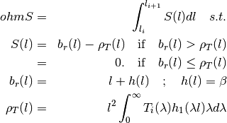
where
 solve the equation
 ;
;  is half the current electrode spacing
  ,
and
,
and  denotes the first-order of the Bessel function of the first
kind,
denotes the first-order of the Bessel function of the first
kind,  is the coordinate value on y-axis direction of the
intercept term of the and ,
is the coordinate value on y-axis direction of the
intercept term of the and ,  resistivity transform function,
  denotes the integral variable,
where n denotes the number of layers,
denotes the integral variable,
where n denotes the number of layers,  and
and  are
the resistivity and thickness of the
are
the resistivity and thickness of the  layer, respectively.
Get more explanations and cleareance of formula in the paper of
`Kouadio et al 2022`_.
layer, respectively.
Get more explanations and cleareance of formula in the paper of
`Kouadio et al 2022`_.References
- Kouadio, K.L., Nicolas, K.L., Binbin, M., Déguine, G.S.P. & Serge,
K.K. (2021, October) Bagoue dataset-Cote d’Ivoire: Electrical profiling, electrical sounding and boreholes data, Zenodo. doi:10.5281/zenodo.5560937
- Koefoed, O. (1970). A fast method for determining the layer distribution
from the raised kernel function in geoelectrical sounding. Geophysical Prospecting, 18(4), 564–570. https://doi.org/10.1111/j.1365-2478.1970.tb02129.x
- Koefoed, O. (1976). Progress in the Direct Interpretation of Resistivity
Soundings: an Algorithm. Geophysical Prospecting, 24(2), 233–240. https://doi.org/10.1111/j.1365-2478.1976.tb00921.x
- Biemi, J. (1992). Contribution à l’étude géologique, hydrogéologique et par télédétection
de bassins versants subsaheliens du socle précambrien d’Afrique de l’Ouest: hydrostructurale hydrodynamique, hydrochimie et isotopie des aquifères discontinus de sillons et aires gran. In Thèse de Doctorat (IOS journa, p. 493). Abidjan, Cote d’Ivoire
- kalfeat.tools.exmath.plot_(*args: List[Union[str, Array, ...]], figsize: Tuple[int] = None, raw: bool = False, style: str = 'seaborn', dtype: str = 'erp', kind: Optional[str] = None, **kws) None[source]
Quick visualization for fitting model, Electrical Resistivity Profiling and Vertical Electrical Sounding curves.
- param x
array-like - array of data for x-axis representation
- param y
array-like - array of data for plot y-axis representation
- param figsize
tuple - Mtplotlib (MPL) figure size; should be a tuple value of integers e.g. figsize =(10, 5).
- param raw
bool- Originally the plot_ function is intended for the fitting Electrical Resistivity Profiling model i.e. the correct value of Electrical Resistivity Profiling data. However, when the raw is set to
True, it plots the both curves: The fitting model as well as the uncorrected model. So both curves are overlaining or supperposed.- param style
str - Pyplot style. Default is
seaborn- param dtype
str - Kind of data provided. Can be Electrical Resistivity Profiling data or Vertical Electrical Sounding data. When the Electrical Resistivity Profiling data are provided, the common plot is sufficient to visualize all the data insignt i.e. the default value of kind is kept to
None. However, when the data collected is Vertical Electrical Sounding data, the convenient plot for visualization is theloglogfor parameter kind` while the dtype can be set to VES to specify the labels into the x-axis. The default value of dtype iserpfor common visualization.- param kind
str - Use to specify the kind of data provided. See the explanation of dtype parameters. By default kind is set to
Nonei.e. its keep the normal plots. It can beloglog,semilogxandsemilogy.- param kws
dict - Additional Matplotlib plot keyword arguments. To cus- tomize the plot, one can provide a dictionnary of MPL keyword additional arguments like the example below.
- Example
>>> import numpy as np
>>> from kalfeat.tools.exmath import plot_
>>> x, y = np.arange(0 , 60, 10) ,np.abs( np.random.randn (6))
>>> KWS = dict (xlabel ='Stations positions', ylabel= 'resistivity(ohm.m)',
            rlabel = 'raw cuve', rotate = 45 )
>>> plot_(x, y, '-ok', raw = True , style = 'seaborn-whitegrid',
          figsize = (7, 7) ,**KWS )
- kalfeat.tools.exmath.power(p: Sub[SP[Array, DType[int]]] | List[int]) float[source]
Compute the power of the selected conductive zone. Anomaly power is closely referred to the width of the conductive zone.
The power parameter implicitly defines the width of the conductive zone and is evaluated from the difference between the abscissa
 and the end
  points of
the selected anomaly:
points of
the selected anomaly:
- Parameters
p – array-like. Station position of conductive zone.
- Returns
Absolute value of the width of conductive zone in meters.
- kalfeat.tools.exmath.quickplot(arr: Array | List[float], dl: float = 10) None[source]
Quick plot to see the anomaly
- kalfeat.tools.exmath.scalePosition(ydata: Array | SP | Series | DataFrame, xdata: Array | Series = None, func: Optional[F] = None, c_order: Optional[int | str] = 0, show: bool = False, **kws)[source]
Correct data location or position and return new corrected location
- Parameters
ydata (array_like, series or dataframe) – The dependent data, a length M array - nominally
f(xdata, ...).xdata (array_like or object) – The independent variable where the data is measured. Should usually be an M-length sequence or an (k,M)-shaped array for functions with k predictors, but can actually be any object. If
None, xdata is generated by default using the length of the given ydata.func (callable) – The model function,
f(x, ...). It must take the independent variable as the first argument and the parameters to fit as separate remaining arguments. The default func islinearfunction i.e forf(x)= ax +b. where a is slope and b is the intercept value. Setting your own function for better fitting is recommended.c_order (int or str) – The index or the column name if
ydatais given as a dataframe to select the right column for scaling.show (bool) – Quick visualization of data distribution.
kws (dict) – Additional keyword argument from scipy.optimize_curvefit parameters. Refer to scipy.optimize.curve_fit.
- Returns
- ydata - array -like - Data scaled
- popt - array-like Optimal values for the parameters so that the sum of
the squared residuals of
f(xdata, \*popt) - ydatais minimized.- pcov - array like The estimated covariance of popt. The diagonals provide
the variance of the parameter estimate. To compute one standard deviation
errors on the parameters use
perr = np.sqrt(np.diag(pcov)). How thesigma parameter affects the estimated covariance depends on absolute_sigma
argument, as described above. If the Jacobian matrix at the solution
doesn’t have a full rank, then ‘lm’ method returns a matrix filled with
np.inf, on the other hand ‘trf’ and ‘dogbox’ methods use Moore-Penrose
pseudoinverse to compute the covariance matrix.
Examples
>>> from kalfeat.tools import erpSelector, scalePosition
>>> df = erpSelector('data/erp/l10_gbalo.xlsx')
>>> df.columns
... Index(['station', 'resistivity', 'longitude', 'latitude', 'easting',
'northing'],
dtype='object')
>>> # correcting northing coordinates from easting data
>>> northing_corrected, popt, pcov = scalePosition(ydata =df.northing ,
xdata = df.easting, show=True)
>>> len(df.northing.values) , len(northing_corrected)
... (20, 20)
>>> popt  # by default popt =(slope:a ,intercept: b)
...  array([1.01151734e+00, 2.93731377e+05])
>>> # corrected easting coordinates using the default x.
>>> easting_corrected, *_= scalePosition(ydata =df.easting , show=True)
>>> df.easting.values
... array([790284, 790281, 790277, 790270, 790265, 790260, 790254, 790248,
...       790243, 790237, 790231, 790224, 790218, 790211, 790206, 790200,
...       790194, 790187, 790181, 790175], dtype=int64)
>>> easting_corrected
... array([790288.18571705, 790282.30300999, 790276.42030293, 790270.53759587,
...       790264.6548888 , 790258.77218174, 790252.88947468, 790247.00676762,
...       790241.12406056, 790235.2413535 , 790229.35864644, 790223.47593938,
...       790217.59323232, 790211.71052526, 790205.8278182 , 790199.94511114,
...       790194.06240407, 790188.17969701, 790182.29698995, 790176.41428289])
- kalfeat.tools.exmath.sfi(cz: Sub[Array[T, DType[T]]] | List[float], p: Sub[SP[Array, DType[int]]] | List[int] = None, s: Optional[str] = None, dipolelength: Optional[float] = None, plot: bool = False, raw: bool = False, **plotkws) float[source]
Compute the pseudo-fracturing index known as sfi.
The sfi parameter does not indicate the rock fracturing degree in the underground but it is used to speculate about the apparent resistivity dispersion ratio around the cumulated sum of the resistivity values of the selected anomaly. It uses a similar approach of IF parameter proposed by Dieng et al (2004). Furthermore, its threshold is set to
 for symmetrical anomaly characterized by a perfect
distribution of resistivity in a homogenous medium. The formula is
given by:
for symmetrical anomaly characterized by a perfect
distribution of resistivity in a homogenous medium. The formula is
given by:
where
 and
and  are the anomaly power and the magnitude
respectively.
are the anomaly power and the magnitude
respectively.  is and
  are the projected
power and magnitude of the lower point of the selected anomaly.
are the projected
power and magnitude of the lower point of the selected anomaly.- Parameters
cz – array-like. Selected conductive zone
p – array-like. Station positions of the conductive zone.
dipolelength – float. If p is not given, it will be set automatically using the default value to match the
czsize. The default value is10..plot – bool. Visualize the fitting curve. Default is
False.raw – bool. Overlaining the fitting curve with the raw curve from cz.
plotkws – dict. Matplotlib plot keyword arguments.
- Example
>>> from numpy as np
>>> from kalfeat.properties import P
>>> from kalfeat.tools.exmath import sfi
>>> rang = np.random.RandomState (42)
>>> condzone = np.abs(rang.randn (7))
>>> # no visualization and default value `s` with gloabl minimal rho
>>> pfi = sfi (condzone)
... 3.35110143
>>> # visualize fitting curve
>>> plotkws  = dict (rlabel = 'Conductive zone (cz)',
                     label = 'fitting model',
                     color=f'{P().frcolortags.get("fr3")}',
                     )
>>> sfi (condzone, plot= True , s= 5, figsize =(7, 7),
          **plotkws )
... Out[598]: (array([ 0., 10., 20., 30.]), 1)
References
See Numpy Polyfit
- See Stackoverflow
the answer of AkaRem edited by Tobu and Migilson.
- See Numpy Errorstate and
how to implement the context manager.
- kalfeat.tools.exmath.shape(cz: Array | List[float], s: Optional[str, int] = Ellipsis, p: SP = Ellipsis) str[source]
Compute the shape of anomaly.
The shape parameter is mostly used in the basement medium to depict the better conductive zone for the drilling location. According to Sombo et al. (2011; 2012), various shapes of anomalies can be described such as:
“V”, “U”, “W”, “M”, “K”, “C”, and “H”
The shape consists to feed the algorithm with the Electrical Resistivity Profiling resistivity values by specifying the station
 . Indeed,
mostly,
. Indeed,
mostly,  is the station with a very low resistivity value
expected to be the drilling location.
is the station with a very low resistivity value
expected to be the drilling location.- Parameters
cz – array-like - Conductive zone resistivity values
s – int, str - Station position index or name.
p – Array-like - Should be the position of the conductive zone.
Note
If s is given, p should be provided. If p is missing an error will raises.
- Returns
str - the shape of anomaly.
- Example
>>> import numpy as np
>>> rang = random.RandomState(42)
>>> from kalfeat.tools.exmath import shape_
>>> test_array1 = np.arange(10)
>>> shape_ (test_array1)
...  'C'
>>> test_array2 = rang.randn (7)
>>> _shape(test_array2)
... 'K'
>>> test_array3 = np.power(10, test_array2 , dtype =np.float32)
>>> _shape (test_array3)
... 'K'   # does not change whatever the resistivity values.
References
- Sombo, P. A., Williams, F., Loukou, K. N., & Kouassi, E. G. (2011).
Contribution de la Prospection Électrique à L’identification et à la Caractérisation des Aquifères de Socle du Département de Sikensi (Sud de la Côte d’Ivoire). European Journal of Scientific Research, 64(2), 206–219.
- Sombo, P. A. (2012). Application des methodes de resistivites electriques
dans la determination et la caracterisation des aquiferes de socle en Cote d’Ivoire. Cas des departements de Sikensi et de Tiassale (Sud de la Cote d’Ivoire). Universite Felix Houphouet Boigny.
- kalfeat.tools.exmath.shortPlot(sample, cz=None)[source]
Quick plot to visualize the sample line as well as the selected conductive zone if given.
- Parameters
sample – array_like, the electrical profiling array
cz – array_like, the selected conductive zone. If
None, cz should be plotted.
- Example
>>> import numpy as np
>>> from kalfeat.tools.exmath import shortPlot, define_conductive_zone
>>> test_array = np.random.randn (10)
>>> selected_cz ,*_ = define_conductive_zone(test_array, 7)
>>> shortPlot(test_array, selected_cz )
- kalfeat.tools.exmath.type_(erp: Array[DType[float]]) str[source]
Compute the type of anomaly.
The type parameter is defined by the African Hydraulic Study Committee report (CIEH, 2001). Later it was implemented by authors such as (Adam et al., 2020; Michel et al., 2013; Nikiema, 2012). Type comes to help the differenciation of two or several anomalies with the same shape. For instance, two anomalies with the same shape
Wwill differ from the order of priority of their types. The type depends on the lateral resistivity distribution of underground (resulting from the pace of the apparent resistivity curve) along with the whole Electrical Resistivity Profiling survey line. Indeed, four types of anomalies were emphasized:“EC”, “CB2P”, “NC” and “CP”.
For more details refers to references.
- Parameters
erp – array-like - Array of Electrical Resistivity Profiling line composed of apparent resistivity values.
- Returns
str -The type of anomaly.
- Example
>>> import numpy as np
>>> from kalfeat.tools.exmath import type_
>>> rang = random.RandomState(42)
>>> test_array2 = rang.randn (7)
>>> type_(np.abs(test_array2))
... 'EC'
>>> long_array = np.abs (rang.randn(71))
>>> type(long_array)
... 'PC'
References
- Adam, B. M., Abubakar, A. H., Dalibi, J. H., Khalil Mustapha,M., & Abubakar,
A. H. (2020). Assessment of Gaseous Emissions and Socio-Economic Impacts From Diesel Generators used in GSM BTS in Kano Metropolis. African Journal of Earth and Environmental Sciences, 2(1),517–523. https://doi.org/10.11113/ajees.v3.n1.104
- CIEH. (2001). L’utilisation des méthodes géophysiques pour la recherche
d’eaux dans les aquifères discontinus. Série Hydrogéologie, 169.
- Michel, K. A., Drissa, C., Blaise, K. Y., & Jean, B. (2013). Application
de méthodes géophysiques à l ’ étude de la productivité des forages d ’eau en milieu cristallin : cas de la région de Toumodi ( Centre de la Côte d ’Ivoire). International Journal of Innovation and Applied Studies, 2(3), 324–334.
- Nikiema, D. G. C. (2012). Essai d‘optimisation de l’implantation géophysique
des forages en zone de socle : Cas de la province de Séno, Nord Est du Burkina Faso (IRD). (I. / I. Ile-de-France, Ed.). IST / IRD Ile-de-France, Ouagadougou, Burkina Faso, West-africa. Retrieved from http://documentation.2ie-edu.org/cdi2ie/opac_css/doc_num.php?explnum_id=148
- kalfeat.tools.exmath.vesDataOperator(AB: Array = None, rhoa: Array = None, data: DataFrame = None, typeofop: str = None, outdf: bool = False) Tuple[Array] | DataFrame[source]
Check the data in the given deep measurement and set the suitable operations for duplicated spacing distance of current electrodes AB.
Sometimes at the potential electrodes (MN), the measurement of AB are collected twice after modifying the distance of MN a bit. At this point, two or many resistivity values are targetted to the same distance AB (AB still remains unchangeable while while MN is changed). So the operation consists whether to average (
mean) the resistiviy values or to take themedianvalues or toleaveOneOut(i.e. keep one value of resistivity among the different values collected at the same point`AB`) at the same spacing AB. Note that for the LeaveOneOut`, the selected resistivity value is randomly chosen.- Parameters
AB – array-like - Spacing of the current electrodes when exploring in deeper. Units are in meters.
rhoa – array-like - Apparent resistivity values collected in imaging in depth. Units are in
 not
not 
data – DataFrame - It is composed of spacing values AB and the apparent resistivity values rhoa. If data is given, params AB and rhoa should be kept to
None.typeofop – str - Type of operation to apply to the resistivity values rhoa of the duplicated spacing points AB. The default operation is
mean.outdf – bool - Outpout a new dataframe composed of AB and rhoa data renewed.
- Returns
Tuple of (AB, rhoa): New values computed from typeofop
DataFrame: New dataframe outputed only if
outdfisTrue.
- Note
By convention AB and MN are half-space dipole length which correspond to AB/2 and MN/2 respectively.
- Example
>>> from kalfeat.tools.exmath import vesDataOperator
>>> from kalfeat.tools.coreutils import vesSelector
>>> data = vesSelector (f= 'data/ves/ves_gbalo.xlsx')
>>> len(data)
... (32, 3) # include the potentiel electrode values `MN`
>>> df= vesDataOperator(data.AB, data.resistivity,
                        typeofop='leaveOneOut', outdf =True)
>>> df.shape
... (26, 2) # exclude `MN` values and reduce(-6) the duplicated values.
Module Funcutils
- kalfeat.tools.funcutils.accept_types(*objtypes: list, format: bool = False) List[str] | str[source]
List the type format that can be accepted by a function.
- Parameters
objtypes – List of object types.
format – bool - format the list of the name of objects.
- Returns
list of object type names or str of object names.
- Example
>>> import numpy as np; import pandas as pd
>>> from kalfeat.tools.funcutils import accept_types
>>> accept_types (pd.Series, pd.DataFrame, tuple, list, str)
... "'Series','DataFrame','tuple','list' and 'str'"
>>> atypes= accept_types (
    pd.Series, pd.DataFrame,np.ndarray, format=True )
..."'Series','DataFrame' and 'ndarray'"
- kalfeat.tools.funcutils.check_dimensionality(obj, data, z, x)[source]
Check dimensionality of data and fix it.
- Parameters
obj – Object, can be a class logged or else.
data – 2D grid data of ndarray (z, x) dimensions.
z – array-like should be reduced along the row axis.
x – arraylike should be reduced along the columns axis.
- kalfeat.tools.funcutils.cpath(savepath=None, dpath=None)[source]
Control the existing path and create one of it does not exist.
- Parameters
savepath – Pathlike obj, str
dpath – str, default pathlike obj
- kalfeat.tools.funcutils.format_notes(text: str, cover_str: str = '~', inline=70, **kws)[source]
Format note :param text: Text to be formated.
- Parameters
cover_str – type of
strto surround the text.inline – Nomber of character before going in liine.
margin_space – Must be <1 and expressed in %. The empty distance between the first index to the inline text
- Example
>>> from kalfeat.tools import funcutils as func
>>> text ='Automatic Option is set to ``True``.'            ' Composite estimator building is triggered.'
>>>  func.format_notes(text= text ,
...                       inline = 70, margin_space = 0.05)
- kalfeat.tools.funcutils.is_installing(module, upgrade=True, DEVNULL=False, action=True, verbose=0, **subpkws)[source]
Install or uninstall a module using the subprocess under the hood.
- Parameters
module – str, module name.
:param upgrade:bool, install the lastest version.
:param verbose:output a message.
- Parameters
DEVNULL – decline the stdoutput the message in the console.
action – str, install or uninstall a module.
subpkws – additional subprocess keywords arguments.
- Example
>>> from pycsamt.tools.funcutils import is_installing
>>> is_installing(
    'tqdm', action ='install', DEVNULL=True, verbose =1)
>>> is_installing(
    'tqdm', action ='uninstall', verbose =1)
- kalfeat.tools.funcutils.make_introspection(Obj: object, subObj: Sub[object]) None[source]
Make introspection by using the attributes of instance created to populate the new classes created.
- Parameters
Obj – callable New object to fully inherits of subObject attributes.
subObj – Callable Instance created.
- kalfeat.tools.funcutils.read_from_excelsheets(erp_file: Optional[str] = None) List[DataFrame][source]
Read all Excelsheets and build a list of dataframe of all sheets.
- Parameters
erp_file – Excell workbooks containing erp profile data.
- Returns
A list composed of the name of erp_file at index =0 and the datataframes.
- kalfeat.tools.funcutils.repr_callable_obj(obj: F)[source]
Represent callable objects.
Format class, function and instances objects.
- Parameters
obj – class, func or instances object to format.
- Raises
TypeError - If object is not a callable or instanciated.
- Examples
>>> from kalfeat.tools.funcutils import repr_callable_obj
>>> from kalfeat.methods.dc import (
    ElectricalMethods, ResistivityProfiling)
>>> callable_format(ElectricalMethods)
... 'ElectricalMethods(AB= None, arrangement= schlumberger,
        area= None, MN= None, projection= UTM, datum= WGS84,
        epsg= None, utm_zone= None, fromlog10= False)'
>>> callable_format(ResistivityProfiling)
... 'ResistivityProfiling(station= None, dipole= 10.0,
        auto_station= False, kws= None)'
>>> robj= ResistivityProfiling (AB=200, MN=20, station ='S07')
>>> repr_callable_obj(robj)
... 'ResistivityProfiling(AB= 200, MN= 20, arrangememt= schlumberger,
        utm_zone= None, projection= UTM, datum= WGS84, epsg= None,
        area= None, fromlog10= False, dipole= 10.0, station= S07)'
>>> repr_callable_obj(robj.fit)
... 'fit(data= None, kws= None)'
- kalfeat.tools.funcutils.round_dipole_length(value, round_value=5.0)[source]
small function to graduate dipole length 5 to 5. Goes to be reality and simple computation .
- Parameters
value (float) – value of dipole length
- Returns
value of dipole length rounded 5 to 5
- Return type
float
- kalfeat.tools.funcutils.sPath(name_of_path: str)[source]
Savepath func. Create a path with name_of_path if path not exists.
- Parameters
name_of_path – str, Path-like object. If path does not exist, name_of_path should be created.
- kalfeat.tools.funcutils.savepath_(nameOfPath)[source]
Shortcut to create a folder :param nameOfPath: Path name to save file :type nameOfPath: str
- Returns
New folder created. If the nameOfPath exists, will return
None
:rtype:str
- kalfeat.tools.funcutils.smart_format(iter_obj)[source]
Smart format iterable ob.
- Parameters
iter_obj – iterable obj
- Example
>>> from kalfeat.tools.funcutils import smart_format
>>> smart_format(['model', 'iter', 'mesh', 'data'])
... 'model','iter','mesh' and 'data'
- kalfeat.tools.funcutils.smart_strobj_recognition(name: str, container: List | Tuple | Dict[Any, Any], stripitems: str | List | Tuple = '_', deep: bool = False) str[source]
Find the likelihood word in the whole containers and returns the value.
- Parameters
name – str - Value of to search. I can not match the exact word in
the container :param container: list, tuple, dict- container of the many string words. :param stripitems: str - ‘str’ items values to sanitize the content
element of the dummy containers. if different items are provided, they can be separated by
:,,and;. The items separators aforementioned can not be used as a component in the name. For isntance:name= 'dipole_'; stripitems='_' -> means remove the '_' under the ``dipole_`` name= '+dipole__'; stripitems ='+;__'-> means remove the '+' and '__' under the value `name`.
- Parameters
deep – bool - Kind of research. Go deeper by looping each items for find the initials that can fit the name. Note that, if given, the first occurence should be consider as the best name…
- Returns
Likelihood object from container or Nonetype if none object is detected.
- Example
>>> from kalfeat.tools.funcutils import smart_strobj_recognition
>>> from kalfeat.methods import ResistivityProfiling
>>> rObj = ResistivityProfiling(AB= 200, MN= 20,)
>>> smart_strobj_recognition ('dip', robj.__dict__))
... None
>>> smart_strobj_recognition ('dipole_', robj.__dict__))
... dipole
>>> smart_strobj_recognition ('dip', robj.__dict__,deep=True )
... dipole
>>> smart_strobj_recognition (
    '+_dipole___', robj.__dict__,deep=True , stripitems ='+;_')
... 'dipole'
Module GisTools
- kalfeat.tools.gistools.assert_elevation_value(elevation)[source]
make sure elevation is a floating point number
- kalfeat.tools.gistools.assert_lon_value(longitude)[source]
make sure longitude is in decimal degrees
- kalfeat.tools.gistools.convert_position_float2str(position)[source]
convert position float to a string in the format of DD:MM:SS
- Parameters
**position** (float) – decimal degrees of latitude or longitude
- Returns
**position_str** – latitude or longitude in format of DD:MM:SS.ms
- Return type
string
Example
>>> import mtpy.utils.gis_tools as gis_tools
>>> gis_tools.convert_position_float2str(-118.34563)
- kalfeat.tools.gistools.convert_position_str2float(position_str)[source]
Convert a position string in the format of DD:MM:SS to decimal degrees
- Parameters
**position_str** (string ('DD:MM:SS.ms')) – degrees of latitude or longitude
- Returns
**position** – latitude or longitude in decimal degrees
- Return type
float
Example
>>> import mtpy.utils.gis_tools as gis_tools
>>> gis_tools.convert_position_str2float('-118:34:56.3')
- kalfeat.tools.gistools.get_utm_string_from_sr(spatialreference)[source]
return utm zone string from spatial reference instance
- kalfeat.tools.gistools.get_utm_zone(latitude, longitude)[source]
Get utm zone from a given latitude and longitude
- kalfeat.tools.gistools.ll_to_utm(reference_ellipsoid, lat, lon)[source]
converts lat/long to UTM coords. Equations from USGS Bulletin 1532 East Longitudes are positive, West longitudes are negative. North latitudes are positive, South latitudes are negative Lat and Long are in decimal degrees Written by Chuck Gantz- chuck.gantz@globalstar.com
- Outputs:
UTMzone, easting, northing
- kalfeat.tools.gistools.project_point_ll2utm(lat, lon, datum='WGS84', utm_zone=None, epsg=None)[source]
Project a point that is in Lat, Lon (will be converted to decimal degrees) into UTM coordinates.
- latfloat or string (DD:MM:SS.ms)
latitude of point
- lonfloat or string (DD:MM:SS.ms)
longitude of point
- datumstring
well known datum ex. WGS84, NAD27, NAD83, etc.
- utm_zonestring
zone number and ‘S’ or ‘N’ e.g. ‘55S’
- epsgint
epsg number defining projection (see http://spatialreference.org/ref/ for moreinfo) Overrides utm_zone if both are provided
- proj_point: tuple(easting, northing, zone)
projected point in UTM in Datum
- kalfeat.tools.gistools.project_point_utm2ll(easting, northing, utm_zone, datum='WGS84', epsg=None)[source]
Project a point that is in Lat, Lon (will be converted to decimal degrees) into UTM coordinates.
- eastingfloat
easting coordinate in meters
- northingfloat
northing coordinate in meters
- utm_zonestring (##N or ##S)
utm zone in the form of number and North or South hemisphere, 10S or 03N
- datumstring
well known datum ex. WGS84, NAD27, etc.
- proj_point: tuple(lat, lon)
projected point in lat and lon in Datum, as decimal degrees.
- kalfeat.tools.gistools.project_points_ll2utm(lat, lon, datum='WGS84', utm_zone=None, epsg=None)[source]
Project a list of points that is in Lat, Lon (will be converted to decimal degrees) into UTM coordinates.
- latfloat or string (DD:MM:SS.ms)
latitude of point
- lonfloat or string (DD:MM:SS.ms)
longitude of point
- datumstring
well known datum ex. WGS84, NAD27, NAD83, etc.
- utm_zonestring
zone number and ‘S’ or ‘N’ e.g. ‘55S’. Defaults to the centre point of the provided points
- epsgint
epsg number defining projection (see http://spatialreference.org/ref/ for moreinfo) Overrides utm_zone if both are provided
- proj_point: tuple(easting, northing, zone)
projected point in UTM in Datum
- kalfeat.tools.gistools.utm_to_ll(reference_ellipsoid, northing, easting, zone)[source]
converts UTM coords to lat/long. Equations from USGS Bulletin 1532 East Longitudes are positive, West longitudes are negative. North latitudes are positive, South latitudes are negative Lat and Long are in decimal degrees. Written by Chuck Gantz- chuck.gantz@globalstar.com Converted to Python by Russ Nelson <nelson@crynwr.com>
- Outputs:
Lat,Lon
- kalfeat.tools.gistools.utm_wgs84_conv(lat, lon)[source]
Bidirectional UTM-WGS84 converter https://github.com/Turbo87/utm/blob/master/utm/conversion.py :param lat: :param lon: :return: tuple(e, n, zone, lett)
Package Properties
Module Property
- class kalfeat.property.ElectricalMethods(AB: float = 200.0, MN: float = 20.0, arrangement: str = 'schlumberger', area: Optional[str] = None, projection: str = 'UTM', datum: str = 'WGS84', epsg: Optional[int] = None, utm_zone: Optional[str] = None, fromlog10: bool = False, verbose: int = 0)[source]
Base class of geophysical electrical methods
The electrical geophysical methods are used to determine the electrical resistivity of the earth’s subsurface. Thus, electrical methods are employed for those applications in which a knowledge of resistivity or the resistivity distribution will solve or shed light on the problem at hand. The resolution, depth, and areal extent of investigation are functions of the particular electrical method employed. Once resistivity data have been acquired, the resistivity distribution of the subsurface can be interpreted in terms of soil characteristics and/or rock type and geological structure. Resistivity data are usually integrated with other geophysical results and with surface and subsurface geological data to arrive at an interpretation. Get more infos by consulting this link .
The
kalfeat.methods.electrical.ElectricalMethodscompose the base class of all the geophysical methods that images the underground using the resistivity values.Holds on others optionals infos in
kwsarguments:Attributes
Type
Description
AB
float, array
Distance of the current electrodes in meters. A and B are used as the first and second current electrodes by convention. Note that AB is considered as an array of depth measurement when using the vertical electrical sounding Vertical Electrical Sounding method i.e. AB/2 half-space. Default is ``200``meters.
MN
float, array
Distance of the current electrodes in meters. M and N are used as the first and second potential electrodes by convention. Note that MN is considered as an array of potential electrode spacing when using the collecting data using the vertical electrical sounding Vertical Electrical Sounding method i.e MN/2 halfspace. Default is ``20.``meters.
arrangement
str
Type of dipoles AB and MN arrangememts. Can be schlumberger Wenner- alpha / wenner beta, Gradient rectangular or dipole- dipole. Default is schlumberger.
area
str
The name of the survey location or the exploration area.
fromlog10
bool
Set to
Trueif the given resistivities values are collected on base 10 logarithm.utm_zone
str
string (##N or ##S). utm zone in the form of number and North or South hemisphere, 10S or 03N.
datum
str
well known datum ex. WGS84, NAD27, etc.
projection
str
projected point in lat and lon in Datum latlon, as decimal degrees or ‘UTM’.
epsg
int
epsg number defining projection (see http://spatialreference.org/ref/ for moreinfo). Overrides utm_zone if both are provided.
Notes
The ElectricalMethods consider the given resistivity values as a normal values and not on base 10 logarithm. So if log10 values are given, set the argument fromlog10 value to
True.
- class kalfeat.property.P(hl=None)[source]
Data properties are values that are hidden to avoid modifications alongside the packages. Its was used for assertion, comparison etceteara. These are enumerated below into a property objects.
- frcolortags: Stands for flow rate colors tags. Values are
‘#CED9EF’,’#9EB3DD’, ‘#3B70F2’, ‘#0A4CEF’.
- ididctags: Stands for the list of index set in dictionary which encompasses
key and values of all different prefixes.
isation: List of prefixes used for indexing the stations in the Electrical Resistivity Profiling.
ieasting: List of prefixes used for indexing the easting coordinates array.
inorthing: List of prefixes used to index the northing coordinates.
- iresistivity List of prefix used for indexing the apparent resistivity
values in the Electrical Resistivity Profiling data collected during the survey.
- isren: Is the list of heads columns during the data collections. Any data
head Electrical Resistivity Profiling data provided should be converted into the following arangement:
station
resistivity
easting
northing
- isrll: Is the list of heads columns during the data collections. Any data
head Electrical Resistivity Profiling data provided should be converted into the following arangement:
station
resistivity
longitude
latitude
P: Typing class for fectching the properties.
>>> from kalfeat.property import P
>>> P.idicttags
... <property at 0x1ec1f2c3ae0>
>>> P().idictags
...
{'station': ['pk', 'sta', 'pos'], 'longitude': ['east', 'x', 'long', 'lon'],
 'latitude': ['north', 'y', 'lat'], 'resistivity': ['rho', 'app', 'res']}
>>> {k:v for k, v in  P.__dict__.items() if '__' not in k}
... {'_station': ['pk', 'sta', 'pos'],
     '_easting': ['east', 'x', 'long'],
     '_northing': ['north', 'y', 'lat'],
     '_resistivity': ['rho', 'app', 'res'],
     'frcolortags': <property at 0x1ec1f2fee00>,
     'idicttags': <property at 0x1ec1f2c3ae0>,
     'istation': <property at 0x1ec1f2c3ea0>,
     'ieasting': <property at 0x1ec1f2c39f0>,
     'inorthing': <property at 0x1ec1f2c3c70>,
     'iresistivity': <property at 0x1ec1f2c3e00>,
     'isenr': <property at 0x1ec1f2c3db0>}
>>> P().isrll
... ['station','resistivity','longitude','latitude']
- property frcolortags
set the dictionnary
- property icpr
Keep only the Vertical Electrical Sounding header data …
- property idictcpr
cpr stands for current-potentials and resistivity. They compose the main property values when collected the vertical electrical sounding data.
- property idicttags
Is the collection of data properties
- property ieasting
Use prefix to identify easting coordinates if given in the dataset.
- property ilat
Use prefix to identify latitude coordinates if given in the dataset.
- property ilon
Use prefix to identify longitude coordinates if given in the dataset.
- property inorthing
Use prefix to identify northing coordinates if given in the dataset.
- property iresistivity
Use prefix to identify the resistivity values in the dataset
- property isren
SREN is the abbreviation of S`for ``Stations`,`R``for resistivity, E for
eastingand N fornorthing. SREN is the expected columns in Electrical resistivity profiling. Indeed, it keeps the traditional collections sheets during the survey.
- property isrll
SRLL is the abbreviation of S`for ``Stations`,`R`` for resistivity, L for
Longitudeand L forLatitude. SRLL is the expected columns in Electrical resistivity profiling. Indeed, it keeps the traditional collections sheets during the survey.
- property istation
Use prefix to identify station location positions
- class kalfeat.property.Water(state: str = None, taste: str = 'potable', odor: int | str = 'pure', appearance: str = 'visible', color: str = 'pure white background', capacity: float = 4184.0, vaporization: float = 2257.0, fusion: float = 33.55, density: float = 1.0, magnetism: float = -0.91, miscibility: bool = True, condensation: float = 22, pressure: tuple = (0.6113, Ellipsis, 101.32), compressibility: float = 5.1e-10, triple: tuple = (0.001, 611.657), conductivity: float = 0.05501, melting: float = 0.5, polarity: str = 'bent molecular geometry ', cohesion: str = 'coherent', adhesion: str = 'disambiguation', tension: float = 71.99, action: float = 100.0, issolvent: bool = True, reaction: str = 'amphoteric', ionisation: str = 'hydroxide', tunneling: str = 'hexamer', nommenclature: str = 'oxidane', earthmass: float = 0.23, occurence: float = 0.9739, pH: float | str = 7.0)[source]
- Should be a SuperClass for methods classes which deals with water
properties and components. Instanciate the class shoud raise an error.
Water (H2O) is a polar inorganic compound that is at room temperature a tasteless and odorless liquid, which is nearly colorless apart from an inherent hint of blue. It is by far the most studied chemical compound and is described as the “universal solvent”and the “solvent of life”. It is the most abundant substance on the surface of Earth and the only common substance to exist as a solid, liquid, and gas on Earth’s surface. It is also the third most abundant molecule in the universe (behind molecular hydrogen and carbon monoxide).
The Base class initialize arguments for different methods such as the Electrical Resistivity Profiling and for Vertical Electrical Sounding. The Water should set the attributes and check whether attributes are suitable for what the specific class expects to.
Hold some properties informations:
Property
Description
state
official names for the chemical compound r”$H_2O$”. It can be a matter of
solid,ice,gaseous,water vapororsteam. The default isNone.taste
water from ordinary sources, including bottled mineral water, usually has many dissolved substances, that may give it varying tastes and odors. Humans and other animals have developed senses that enable them to evaluate the potability of water in order to avoid water that is too
saltyorputrid. The default ispotable.odor
Pure water is usually described as tasteless and odorless, although humans have specific sensors that can feel the presence of water in their mouths,and frogs are known to be able to smell it. The default is
pure.color
The color can be easily observed in a glass of tap-water placed against a pure white background, in daylight. The default is
pure white background.appearance
Pure water is visibly blue due to absorption of light in the region ca. 600 nm – 800 nm. The default is
visible.density
Water differs from most liquids in that it becomes less dense as it freezes. In 1 atm pressure, it reaches its maximum density of
1.000 kg/m3(62.43 lb/cu ft) at 3.98 °C (39.16 °F). The default units and values arekg/m3``and ``1.magnetism
Water is a diamagnetic material. Though interaction is weak, with superconducting magnets it can attain a notable interaction. the default value is
 ”. Note that the magnetism
succeptibily has no unit.
”. Note that the magnetism
succeptibily has no unit.capacity
stands for heat capacity. In thermodynamics, the specific heat capacity (symbol cp) of a substance is the heat capacity of a sample of the substance divided by the mass of the sample. Water has a very high specific heat capacity of 4184 J/(kg·K) at 20 °C (4182 J/(kg·K) at 25 °C).The default is is ``4182 ``
vaporization
stands for heat of vaporization. Indeed, the enthalpy of vaporization (symbol
 ), also
known as the (latent) heat of vaporization or heat of
evaporation, is the amount of energy (enthalpy) that
must be added to a liquid substance to transform a
quantity of that substance into a gas. Water has a high
heat of vaporization i.e. 40.65 kJ/mol or 2257 kJ/kg
at the normal boiling point), both of which are a
result of the extensive hydrogen bonding between its
molecules. The default is
), also
known as the (latent) heat of vaporization or heat of
evaporation, is the amount of energy (enthalpy) that
must be added to a liquid substance to transform a
quantity of that substance into a gas. Water has a high
heat of vaporization i.e. 40.65 kJ/mol or 2257 kJ/kg
at the normal boiling point), both of which are a
result of the extensive hydrogen bonding between its
molecules. The default is 2257 kJ/kg.fusion
stands for enthalpy of fusion more commonly known as latent heat of water is 333.55 kJ/kg at 0 °C. The default is
33.55.miscibility
Water is miscible with many liquids, including ethanol in all proportions. Water and most oils are immiscible usually forming layers according to increasing density from the top. default is
True.condensation
As a gas, water vapor is completely miscible with air so the vapor’s partial pressure is 2% of atmospheric pressure and the air is cooled from 25 °C, starting at about 22 °C, water will start to condense, defining the dew point, and creating fog or dew. The default is the degree of condensation set to
22°C.pressure
stands for vapour pressure of water. It is the pressure exerted by molecules of water vapor in gaseous form i.e. whether pure or in a mixture with other gases such as air. The vapor pressure is given as a list from the temperature T, 0°C (0.6113kPa) to 100°C(101.3200kPa). default is
(0.611, ..., 101.32).compressibility
The compressibility of water is a function of pressure and temperature. At 0 °C, at the limit of zero pressure, the compressibility is
5.1x10^−10 P^{a^−1}. The default value is the value at 0 °C.triple
stands for triple point. The temperature and pressure at which ordinary solid, liquid, and gaseous water coexist in equilibrium is a triple point of water. The triple point are set to (.001°C,611.657 Pa) and (100 , 101.325kPa) for feezing (0°C) and boiling point (100°C) points. In addition, the triple point can be set as
(20. , 101.325 kPa)for 20°C. By default, the triple point solid/liquid/vapour is set to(.001, 611.657 Pa ).melting
stands for melting point. Water can remain in a fluid state down to its homogeneous nucleation point of about 231 K (−42 °C; −44 °F). The melting point of ordinary hexagonal ice falls slightly under moderately high pressures, by 0.0073 °C (0.0131 °F)/atm[h] or about
0.5 °C(0.90 °F)/70 atm considered as the default value.conductivity
In pure water, sensitive equipment can detect a very slight electrical conductivity of 0.05501 ± 0.0001 μS/cm at 25.00 °C. default is
.05501.polarity
An important feature of water is its polar nature. The structure has a bent molecular geometry for the two hydrogens from the oxygen vertex. The default is
bent molecular geometryorangular or V-shaped. Other possibility iscovalent bonds `` ``VSEPR theoryfor Valence Shell Electron Repulsion.cohesion
stands for the collective action of hydrogen bonds between water molecules. The default is
coherentfor the water molecules staying close to each other. In addition, the cohesion refers to the tendency of similar or identical particles/surfaces to cling to one another.adhesion
stands for the tendency of dissimilar particles or surfaces to cling to one another. It can be
chemical adhesion,dispersive adhesion,diffusive adhesionanddisambiguation. The default isdisambiguation.tension
stands for the tendency of liquid surfaces at rest to shrink into the minimum surface area possible. Water has an unusually high surface tension of 71.99 mN/m at 25 °C[63] which is caused by the strength of the hydrogen bonding between water molecules. This allows insects to walk on water. The default value is to
71.99 mN/m at 25 °C.action
stands for Capillary action. Water has strong cohesive and adhesive forces, it exhibits capillary action. Strong cohesion from hydrogen bonding and adhesion allows trees to transport water more than 100 m upward. So the default value is set to ``100.``meters.
issolvent
Water is an excellent solvent due to its high dielectric constant. Substances that mix well and dissolve in water are known as hydrophilic (“water-loving”) substances, while those that do not mix well with water are known as hydrophobic (“water-fearing”) substances.
tunnelling
stands for quantum tunneling. It is a quantum mechanical phenomenon whereby a wavefunction can propagate through a potential barrier. It can be
monomersfor the motions which destroy and regenerate the weak hydrogen bond by internal rotations, orhexamerinvolving the concerted breaking of two hydrogen bond. The default ishexamerdiscovered on 18 March 2016.reaction
stands for acide-base reactions. Water is
amphoterici.e. it has the ability to act as either an acid or a base in chemical reactions.ionization
In liquid water there is some self-ionization giving
hydroniumions andhydroxideions. default ishydroxide.earthmass
stands for the earth mass ration in “ppm” unit. Water is the most abundant substance on Earth and also the third most abundant molecule in the universe after the
 . The default
value is ``0.23``ppm of the earth’s mass.
. The default
value is ``0.23``ppm of the earth’s mass.occurence
stands for the abundant molecule in the Earth. Water represents
97.39%of the global water volume of 1.38×10⁹ km3 is found in the oceans considered as the default value.pH
stands for Potential of Hydrogens. It also shows the acidity in nature of water. For instance the “rain” is generally mildly acidic, with a pH between 5.2 and 5.8 if not having any acid stronger than carbon dioxide. At neutral pH, the concentration of the hydroxide ion (
 ) equals that of the (solvated) hydrogen
ion(
) equals that of the (solvated) hydrogen
ion( ), with a value close to
 10^−7 mol L^−1at 25 °C. The default is7.orneutralor the name of any substance pH close to.nommenclature
The accepted IUPAC name of water is
oxidaneor simplywater.Oxidaneis only intended to be used as the name of the mononuclear parent hydride used for naming derivatives of water by substituent nomenclature. The default name isoxidane.Water (chemical formula H2O) is an inorganic, transparent, tasteless, odorless, and nearly colorless chemical substance, which is the main constituent of Earth’s hydrosphere and the fluids of all known living organisms (in which it acts as a solvent). It is vital for all known forms of life, even though it provides neither food, energy, nor organic micronutrients. Its chemical formula, H2O, indicates that each of its molecules contains one oxygen and two hydrogen atoms, connected by covalent bonds. The hydrogen atoms are attached to the oxygen atom at an angle of 104.45°. “Water” is the name of the liquid state of H2O at standard temperature and pressure.
Module Typing
kalfeat Type variables
Some customized type variables need to be explained for easy understanding in the whole package. Indeed, customized type hints is used to define the type of arguments.
- M: Suppose to be the interger variable IntVar to denote the number of
rows in the
Array.- N: Like the
M, N means the number of column in theArray. It is bound with integer variable.
- T: Is known as generic type standing for Any type of variable. We keep
it unchanged.
- U: Unlike T, U stands for nothing. Use to sepcify the one dimentional
array. For instance:
>>> import numpy as np
>>> array = np.arange(4).shape
... (4, )
- S: Indicates the Shape status. It is bound by M, U, N. ‘U’ stands
for nothing for one dimensional array. While, the common shape expects for one of two dimensional arrays, it is possible to extend array for more than one dimensional. The class object
AddShapeis created to grand all the remaining value of integers shape.
D: Stands for dtype object. It is bound with DType.
- Array: Defined for one dimensional array and DType can be specify. For
instance, we generated two arrays (arr1`and `arr2) for different types:
>>> import numpy as np
>>> from kalfeat.typing import TypeVar, Array, DType
>>> T = TypeVar ('T', float)
>>> A = TypeVar ('A', str, bytes )
>>> arr1:Array[T, DType[T]] = np.arange(21) # dtype ='float'
>>> arr2: Array[A, DType[A]] = arr1.astype ('str') # dtype ='str'
- NDArray: Stands for multi-dimensional arrays i.e more than two. Here, the
difference between the one dimensional type variable
Arrayis that while the latter accepts theDTypeargument as the second parameter. It could be turn to the number of multidimentional rows including the `Array as first argument and specify the DType as the second argument like this:>>> import numpy as np >>> from kalfeat.typing import TypeVar, Array, NDarray, DType >>> T =TypeVar ('T', int) >>> U = TypeVar ('U') >>> multidarray = np.arange(7, 7).astype (np.int32) >>> def accept_multid( arrays: NDArray[Array[T, U], DType [T]]= multidarray ): ''' asserted with MyPy and work-fine.''' ...
- Sub: Stands for subset. Indeed, the class is created to define the
conductive zone. It is a subset
SubofArray. For example, we first build an array secondly extract the conductive zone from Electrical Resistivity Profiling line. Finally, we checked the type hint to assert whether the extracted zone is a subset of the whole Electrical Resistivity Profiling line. The demo is given below:>>> import numpy as np >>> from kalfeat.typing import TypeVar, DType, Array , Sub >>> from kalfeat.tools.exmath import _define_conductive_zone >>> T= TypeVar ('T', float) >>> erp_array: Array[T, DType[T]] = np.random.randn (21) # whole line >>> select_zone, _ = _define_conductive_zone (erp = erp_array , auto =True) >>> select_zone: Array[T, DType[T]] >>> def check_cz (select_zone: Sub[Array]): ''' assert with MyPy and return ``True`` as it works fine. ''' ...
- SP: Stands for Station positions. The unit of position may vary, however,
we keep for
kalfeat.method.electrical.ElectricalResistivityProfilingthe default unit inmetersby starting at position 0. Typically, positions are recording according to the dipole length. For the example, we can generated a position values for121 stationswith dipole length equals to50mi.e the length of the survey line is6 km. Here we go:Import required modules and generate the whole survey line:
>>> import numpy as np
>>> from kalfeat.typing import TypeVar, DType, SP, Sub
>>> T =TypeVar ('T', bound =int)
>>> surveyL:SP = np.arange(0, 50 *121 , 50.).astype (np.int32)
... (work fine with MyPy )
- Let’s verify whether the extract data from surveyL is also a subset
of station positions:
- We use the following fonction to to extract the specific
part of whole survey line surveyL:
>>> from kalfeat.tools.exmath import define_conductive_zone
>>> subpos,_ = define_conductive_zone (surveyL, s='S10')
- Now, we check the instance value subpos as subset array of
of SP. Note that the station ‘S10’ is included in the extracted locations and is extented for seven points. For further details, refer to define_conductive_zone.__doc__:
>>> def checksup_type (sp: Sub[SP[T, DType[T]]] = subpos ):
        ''' SP is an array of positions argument `sp`
        shoud be asserted as a subestof the whole line.'''
        ...
... (test verified. subpos is a subset of `SP`)
- Series: Stands for pandas Series object rather than using the specific
pandas.Serieseverywhere in the package.- DataFrame: Likewise the
Seriesgeneric type hint, it stands for pandas DataFrame`_ object. It used to replace ``pandas.DataFrameobject to identify the callable arguments in the whole packages. Both can be instanciated as below:>>> import numpy as np >>> import pandas pd >>> from kalfeat.typing import TypeVar , Any, DType , Series, DataFrame >>> T =TypeVar('T') >>> seriesStr = pd.Series ([f'obx{s}' for s in range(21)], name ='stringobj') >>> seriesFloat = pd.Series (np.arange(7).astype(np.float32), name =floatobj) >>> SERs = Series [DType[str]] # pass >>> SERf =Series [DType [float]] # pass .. >>> dfStr= pd.DataFrame {'ser1':seriesStr , 'obj2': [f'none' for i in range (21)]} >>> dfFloat= pd.DataFrame {'ser1':seriesFloat , 'obj2': np.linspace (3, 28 , 7)} >>> dfAny= pd.DataFrame {'ser1':seriesStr, 'ser2':seriesFloat} >>> DFs = DataFrame [SERs] | DataFrame [DType[str]] >>> DFf = DataFrame [SERf] | DataFrame [DType[float]] >>> DFa = DataFrame [Series[Any]] | DataFrame [DType[T]]
—
Additional definition for common arguments
To better construct a hugue API, an explanation of some argument is useful to let the user aware when meeting such argument in a callable function.
- erpStand for Electrical Resistivity Profiling. Typically, the type hint
for Electrical Resistivity Profiling is
Array[float, DType [float]]orList[float]. Its array is supposed to hold the apparent resistivy values collected during the survey.- p: Typically mean position but by preference means station location
positions. The type hint used to defined the p is ``
Array[int, DType [int]]orList[int]. Indeed, the position supposed to be on integer array and the given values enven in float should be casted to integers.- cz: Stands for Conductive Zone. It is a subset of Electrical Resistivity Profiling so they share the
same type hint. However, for better demarcation,
Subis convenient to use to avoid any confusion about the full Electrical Resistivity Profiling and the extracted conductive as demontrated in the example above inSubtype hint definition.
- class kalfeat.typing.AddShape(*args, **kwds)[source]
Suppose to be an extra bound to top the Shape for dimensional more than two.
Example
>>> import numpy as np
>>> np.random.randn(7, 3, 3)
>>> def check_valid_type (
    array: NDArray [Array[float], Shape[M, AddShape[N]]]):
    ...
- class kalfeat.typing.Array(*args, **kwds)[source]
Arry Type here means the 1D array i.e singular column.
- class kalfeat.typing.DType(*args, **kwds)[source]
DType can be Any Type so it holds ‘T’ type variable.
- class kalfeat.typing.DataFrame(*args, **kwds)[source]
Type hint variable to illutsrate the pandas DataFrame object.
Indeed, pandas DataFrame can be considered as an aggregation of Series, thus, the generic type hint variable is supposed to hold a Series object.
- Example
>>> import numpy as np
>>> import pandas as pd
>>> from kalfeat.typing import DType, DataFrame
- class kalfeat.typing.F(*args, **kwds)[source]
Generic class dedicated for functions, methods and class and return the given types i.e callable object with arguments or Any.
- Example
>>> import functools
>>> def decorator (appender ='get only the documention and pass.'):
        @functools.wraps(func):
        def wrapper(*args, **kwds)
            func.__doc__ = appender + func.__doc__
            return func (*args, **kwds)
        return wrapper
>>> @decorator  # do_nothing = decorator (anyway)
    def anyway(*args, **kwds):
        ''' Im here to '''
        ...
>>> def check_F(anyway:F):
        pass
- class kalfeat.typing.NDArray(*args, **kwds)[source]
NDarray has
M``rows, ``N-columns, Shape and DType object. and Dtype. Shape is unbound for this class since it does not make since to sepecify more integers. However, DType seems useful to provide.- Example
>>> import numpy as np
>>> T= TypeVar (T, str , float) # Dtype here is gone to be "str"
>>> array = np.c_[np.arange(7), np.arange(7).astype ('str')]
>>> def test_array (array: NDArray[T, DType [T]]):...
- class kalfeat.typing.SP(*args, **kwds)[source]
Station position arrays hold integer values of the survey location. Most likely, the station position is given according to the dipole length. Assume the dipole length is
10 metersand survey is carried out on 21 stations. The station position array should be an array of interger values from 0. to 200 meters. as like:>>> import numpy as np >>> positions: SP = np.arange(0, 21 * 10, 10. ).astype (np.int32) # integer values
- class kalfeat.typing.Series(*args, **kwds)[source]
To reference the pandas Series object.
- Example
>>> import numpy as np
>>> import pandas as pd
>>> from kalfeat.typing import DType, Series
>>> ser = pd.Series (np.arange (21), name ='nothing')
- class kalfeat.typing.Shape(*args, **kwds)[source]
Generic to construct a tuple shape for NDarray. Shape has is written wait for two dimensional arrays with M-row and N-columns. However for three dimensional,`Optional` Type could be:
- Example
>>> import numpy as np
>>> # For 1D array
>>> np
>>> np.random.rand(7)
>>> def check_array1d(
    array: Array[float, Shape[M, None]])
>>> np.random.rand (7, 7).astype('>U12'):
>>> def check_array2d_type (
    array: NDArray[Array[str], Shape [M, N], DType ['>U12']])
Module Exceptions
Module Docs
Module Decorators
- class kalfeat.decorators.deprecated(reason)[source]
Used to mark functions, methods and classes deprecated, and prints warning message when it called decorators based on https://stackoverflow.com/a/40301488 .
Author: YingzhiGou Date: 20/06/2017
- class kalfeat.decorators.docAppender(func0: Callable[[F], F], from_: str = 'Parameters', to: str = 'Returns', insertfrom: str = 'Parameters', remove=True)[source]
Decorator to generate a new doctring from appending the other class docstrings.
Indeed from the startpoint <from_> and the endpoint<to>, one can select the part of the any function or class doctrings to append to the existing doctring for a new doctring creation. This trip is useful to avoid redundancing parameters definitions everywhere in the scripts.
- Parameters
func0 (callable,) – Function or class to collect the doctring from.
from (str) – Reference word or expression to start the collection of the necessary doctring from the func0. It is the startpoint. The default is
Parameters.to (str) – Reference word to end the collection of the necessary part of the docstring of func0. It is the endpoint. The default is
Returns.insert (str,) – Reference word or expression to insert the collected doctring from the func0 and append of the index of the insert word in func. If not found in the func doctring, it should retun None so nothing should be appended. The default is
Parameters.
Examples
>>> from kalfeat.decorators import docAppender
>>> def func0 (*args, **kwargs):
...        '''Im here so share my doctring.
...
...        Parameters
...        -----------
...        * args: list,
...            Collection of the positional arguments
...        ** kwargs: dict
...            Collection of keywords arguments
...        Returns
...        -------
...             None: nothing
...        '''
...        pass
>>> def func(s, k=0):
...        ''' Im here to append the docstring from func0
...        Parameters
...        ----------
...        s: str ,
...            Any string value
...        k: dict,
...            first keyword arguments
...
...        Returns
...        --------
...            None, I return nothing
...        '''
>>> deco = docAppender(func0 , from_='Parameters',
...                        to='Returns', insert ='---\n')(func)
>>> deco.__doc__
...
Warning
Be sure to append two doctrings with the same format. One may choose either the sphinx or the numpy doc formats. Not Mixing the both.
- class kalfeat.decorators.docSanitizer[source]
Decorator to clean the doctring and set all values of sections to the same level.
It sanitizes the doctring for the use of sphinx documentation.
Examples
>>> from kalfeat.decorators import docSanitizer
>>> def messdocfunc():
...        '''My doctring is mess. I need to be polished and well arranged.
...
...        Im here to sanitize the mess doctring.
...
...        Parameters
...        ----------
...                * args: list,
...                    Collection of the positional arguments
...                ** kwargs: dict
...                    Collection of keywords arguments
...
...        * kwargs: list,
...        Collection of the keyword arguments
...
...        Warnings
...        --------
...        Let check for warnings string ...
...
...       '''
...       pass
>>> cleandocfunc = docSanitizer()(messfocfunc)
>>> print(cleandocfunc.__doc__)
... '''
...    My doctring is mess. I need to be polished and well arranged.
...
...    Parameters
...    ----------
...    * args: list,
...       Collection of the positional arguments
...    ** kwargs: dict
...        Collection of keywords arguments
...    * kwargs: list,
...        Collection of the keyword arguments
...    '''
- class kalfeat.decorators.docstring(func0, start='Parameters', end=None)[source]
Generate new doctring of a function or class by appending the doctring of another function from the words considered as the startpoint start to endpoint end.
Sometimes two functions inherit the same parameters. Repeat the writing of the same parameters is redundancy. So the most easier part is to collect the doctring of the inherited function and paste to the new function from the startpoint.
- Parameters
func0 (callable,) – function to use its doctring
start (str) – Value from which the new docstring should be start.
end (str) – endpoint Value of the doctring. Stop considering point.
Examples
>>> from kalfeat.decorators import writedf , predPlot, docstring
>>> docs = doctring(writedf, start ='param reason', end='param to_')(predPlot)
>>> docs.__doc__
>>> predPlot.__doc__ # doc modified and holds the writedf docstring too.
Author: @Daniel03 Date: 18/09/2021
- class kalfeat.decorators.redirect_cls_or_func(*args, **kwargs)[source]
Used to redirected functions or classes. Deprecated functions or class can call others use functions or classes.
Use new function or class to replace old function method or class with multiple parameters.
Author: @Daniel03 Date: 18/10/2020
- class kalfeat.decorators.refAppender(docref=None)[source]
Append the module docstring with reStructured Text references.
Indeed, when a func is decorated, it will add the reStructured Text references as an appender to its reference docstring. So, sphinx can auto-retrieve some replacing values found inline from the kalfeat.documentation.
- Parameters
docref (str) – Reference of the documentation for appending.
Examples
>>> from kalfeat.documentation import __doc__
>>> from kalfeat.tools import decorators
>>> def donothing ():
        ''' Im here to just replace the `|VES|` and `|RES|` values by their
        real meanings.'''
        pass
>>> decorated_donothing = decorators.refAppender(__doc__)(donothing)
>>> decorated_donothing.__doc__
... #new doctring appended and `|VES|` and `|ERP|` are replaced by
... #Vertical Electrical Sounding and Electrical resistivity profiling
... #during compilation in ReadTheDocs.
- kalfeat.decorators.rpop(listitem)[source]
remove all blank line in the item list. :param listitem: list- list of the items and pop all the existing blanck lines.
- class kalfeat.decorators.writef(reason: Optional[str] = None, from_: Optional[str] = None, to: Optional[str] = None, savepath: Optional[str] = None, **kws)[source]
Used to redirected functions or classes. Deprecated functions or class can call others use functions or classes.
Decorate function or class to replace old function method or class with multiple parameters and export files into many other format. .xlsx , .csv or regular format. Decorator mainly focus to export data to other files. Exported file can regular file or excel sheets.
- Parameters
reason – Explain the “What to do?”. Can be write or convert.
from (str
dforregular) – Can bedforregular. Ifdf, func is called and collect its input argguments and write to appropriate extension. If from_`is ``regular`, Can be a simple data put on list of string ready to output file into other format.to – Exported file extension. Can be excel sheeet (.xlsx, csv) or other kind of format.
savepath – Give the path to save the new file written.
Author: @Daniel03 Date: 09/07/2021
Module Logger
kalfeat Logger
Module to track bugs and issues, and also deal with all exceptions in
exceptions.
- class kalfeat._kalfeatlog.kalfeatlog[source]
Field to logs kalfeat module Files in order to tracks all exceptions.
- static get_kalfeat_logger(loggername='')[source]
create a named logger (try different) :param loggername: the name (key) of the logger object in this Python interpreter. :return:
- static load_configure(path2configure=None, OwnloggerBaseConf=False)[source]
configure/setup the logging according to the input configfile
- Parameters
configfile – .yml, .ini, .conf, .json, .yaml.
Its default is the logging.yml located in the same dir as this module. It can be modified to use env variables to search for a log config file.
- static load_configure_set_logfile(path2configfile=None)[source]
configure/setup the logging according to the input configure .yaml file.
- Parameters
configfile – .yml, or add ownUsersConfigYamlfile (*.yml)
Its default is the logging.yml located in logfiles folder It can be modified to use env variables to search for a log config file.